library(terra)
library(tidyverse)
library(tmap)
library(kableExtra)
library(stars)Question & Motivation
How did the 2021 severe winter storm disproportionately affect disadvantaged communities in Houston, Texas?
The February 2021 winter storm triggered a widespread power outage in Texas, leaving many without heat or electricity. However, the impacts of this crisis were not felt equally. Long-standing disparities in housing quality, infrastructure, and socioeconomic conditions affected which neighborhoods were vulnerable to blackouts. This blog post investigates how these inequities influenced outages in Houston, using geospatial data to better understand how disadvantaged communities were disproportionately affected by the storm.
Background
Severe weather events are increasing in frequency and intensity as anthropogenic climate change worsens (NASA, 2021). In Februaray 2021, a severe winter storm swept through the United States and caused a major power crisis in Houston, Texas. Additionally, it is documented that areas in Houston with lower median household income were disproportionately affected and experienced more blackouts (Lee et al., 2022). Since utilties do not release house-level outage information, there is no official documentation showing exactly which homes lost power or which communities were affected. Using publicly available satellite night lights, building polygons, and socioeconomic indicators, this analysis will investigate winter storm Uri and the resulting socioeconomic impacts.
Data
Night lights: Data used is from February 7th & 16th, 2021, showing the before and after of the February 2021 Texas winter storm. The Visible Infrared Imaging Radiometer Suite (VIIRS) data is from NASA’s Level-1 and Atmospheric Archive & Distribution System Distributed Active Archive Center (LAADS DAAC). The .tif files were downloaded and prepared by the instructors. LAADS DAAC Website
Roads: From Geofabrik downloads site where OpenStreetMap (OSM) data can be extracted. This dataset contains geometries for major highways and streets in the Houston area. Used to account for night light interference from highway light pollution. Geofabrik Website
Buildings: Also from Geofabrik, data contained are polygons for houses, commercial structures, and other buildings in the Houston area. Used to calculate an estimate of residential homes impacted by blackouts.
Socio-economic: Obtained from the U.S. Census Bureau’s American Community Survey for census tracts in 2019. This data contains variables like income, race, age, and other demographic information. Used for combining census attribute data to OSM geospatial data to evaluate which communities were impacted by the storm.
Analysis
Packages used in this analysis.
Night Light Intensity Before & After the Storm
There are four night-lights data files used in this analysis. One pair of tiles is for before the storm, February 7th, 2021 and the second pair of tiles is for after the storm, February 16th, 2021. Since Houston sits on the border of two tiles, two tiles per day are needed.
Code
# Load lights data
lights_07_1 <- read_stars(here::here('data', 'VNP46A1', 'VNP46A1.A2021038.h08v05.001.2021039064328.tif'))

lights_07_2 <- read_stars(here::here('data', 'VNP46A1', 'VNP46A1.A2021038.h08v06.001.2021039064329.tif'))

lights_16_1 <- read_stars(here::here('data', 'VNP46A1', 'VNP46A1.A2021047.h08v05.001.2021048091106.tif'))

lights_16_2 <- read_stars(here::here('data', 'VNP46A1', 'VNP46A1.A2021047.h08v06.001.2021048091105.tif'))
Code
# Merge Feb 7th rasters
lights_07 <- st_mosaic(lights_07_1, lights_07_2)

# Merge Feb 16th rasters
lights_16 <- st_mosaic(lights_16_1, lights_16_2)
Before cropping to the Houston area, the Coordinate Reference Systems (CRS) of the bounding box & the night-lights rasters must match.
Code
# Create Houston bounding box
houston_bbox <- st_bbox(c(xmin = -96.5,xmax = -94.5, ymin = 29, ymax = 30.5),
                          crs = "EPSG:4326")

# CRS check before cropping
if (st_crs(houston_bbox) == st_crs(lights_07)){
  print("CRS Match. Ready to crop.")
} else {
  warning("Converting Houston bbox to lights CRS:\n", st_crs(lights_07))

  houston_bbox <- st_transform(houston_bbox, crs = st_crs(lights_07))
}
[1] "CRS Match. Ready to crop."Code
# Crop 07 raster
cropped_07 <- st_crop(lights_07, houston_bbox)
# Crop 16 raster
cropped_16 <- st_crop(lights_16, houston_bbox)
Ready to plot night-lights.
Code
# Plot before & after maps
map_07 <- tm_shape(cropped_07) +
  tm_raster(col.scale = tm_scale_continuous(values = '-brewer.greys'),
            col.legend = tm_legend(show = TRUE,
                                   title = expression(Luminance ~ (Nw ~ cm^{-2} ~ sr^{-1})),
                                   orientation = 'landscape',
                                   width = 42)) +
tm_title(text = "Houston lights before storm (Feb. 7th)",
         position = c(0.03, 1),
         color = "white")

map_16 <- tm_shape(cropped_16) +
  tm_raster(col.scale = tm_scale_continuous(values = '-brewer.greys'),
            col.legend = tm_legend(show = TRUE,
                                   title = expression(Luminance ~ (Nw ~ cm^{-2} ~ sr^{-1})),
                                   orientation = 'landscape')) +
tm_title(text = "Houston lights after storm (Feb. 16th)",
         position = c(0.03, 1),
         color = "white") +
tm_compass(position = c('left', 'bottom'),
           size = 3,
           text.size = 0.9,
           color.dark = 'grey50',
           text.color = 'white') +
tm_scalebar(position = c('left', 'bottom'),
            text.size = 0.8,
            color.dark = 'grey50',
            text.color = 'white')

tmap_arrange(map_07, map_16, nrow = 1)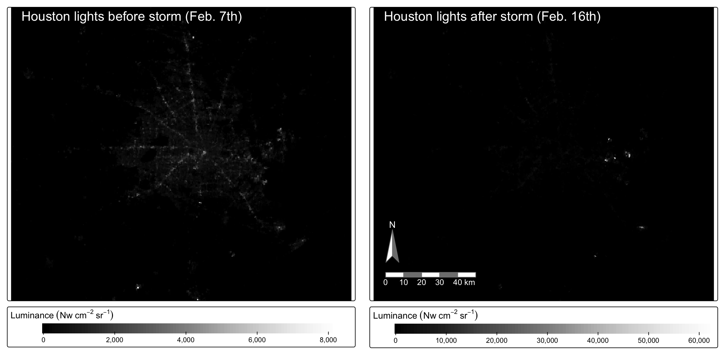
Identify Blackout Areas
To find places that had blackouts, a mask should be created that indicates whether a cell in the lights raster had a blackout or not.
- First, find the change in night-light intensity
Code
# Get raster difference
lights_diff <- cropped_16 - cropped_07- Second, assign
NAto cells that experienced a change greater than -200 nW cm-2sr-1.
Code
# Create houston blackout mask
lights_diff[lights_diff > -200] <- NA- Values in the raster are now only < -200, indicating a significant drop in luminosity.
- Last, the raster will need to be converted to an
sfobject for spatial operations later.
Code
# Vectorize mask
blackout_areas <- lights_diff |>
  st_as_sf() |>
  st_make_valid() |>
  st_transform("EPSG:3083") # Re-project to new crs

# Rename first column name
colnames(blackout_areas)[1] <- "light_difference"
Exclude Highways from Blackout Areas
Code
# Load roads data but only highways with SQL query
roads <- st_read(here::here('data', 'gis_osm_roads_free_1.gpkg'), query = "SELECT * FROM gis_osm_roads_free_1 WHERE fclass='motorway'", quiet = TRUE) |>
  st_transform("EPSG:3083")
Here, we use the road data to account for the influence of light pollution on blackout detection. Major highways produce significant lighting that can interfere with night light differences so only highway segments tagged as motorway are selected for analysis. As a result, locations within 200 meters of highways should be excluded.
Code
# Create 200m buffer
roads_buffer <- st_buffer(roads, dist = 200)
Ensure CRS match between roads and blackout areas.
Code
# Combine road geometries first
roads_buffer_union <- st_union(roads_buffer)

# CRS check before finding difference
if (st_crs(blackout_areas) == st_crs(roads_buffer_union)){
  print("CRS Match. Ready to find difference.")
} else {
  warning("Converting blackout_areas to roads CRS:\n", st_crs(roads_buffer_union))

  blackout_areas <- st_transform(blackout_areas, crs = st_crs(roads_buffer_union))
}
[1] "CRS Match. Ready to find difference."Code
# Find areas NOT within buffer
blackout_far_areas <- st_difference(blackout_areas, roads_buffer_union)
Identify Homes Impacted by Blackouts
Next, we’ll use the homes data to identify homes within our previously defined blackout areas. This enables us to retrieve an estimated number of homes that lost power and a map of impacted homes.
Code
# Read homes data with SQL query
homes <- st_read(
  here::here("data", "gis_osm_buildings_a_free_1.gpkg"),
  query = "
    SELECT * FROM gis_osm_buildings_a_free_1
    WHERE (type IS NULL AND name IS NULL)
       OR type IN ('residential', 'apartments', 'house', 'static_caravan', 'detached')", quiet = TRUE) |>
  st_transform("EPSG:3083")
Ensure CRS match between homes and blackout areas (excluding highways).
Code
# CRS check before filtering
if (st_crs(homes) == st_crs(blackout_far_areas)){
  print("CRS Match. Ready to filter.")
} else {
  warning("Converting homes to blackout_far_areas CRS:\n", st_crs(blackout_far_areas))

  homes <- st_transform(homes, crs = st_crs(blackout_far_areas))
}
[1] "CRS Match. Ready to filter."Code
# Find homes in blackout areas
homes_blackout <- homes |>
  st_filter(y = st_union(blackout_far_areas))
Code
tm_shape(homes_blackout) +
  tm_polygons(col = 'blue') +
  tm_basemap('CartoDB.VoyagerNoLabels') +
  tm_graticules(x = seq(-96.4, -94.8, 0.4), alpha = 0.2) +

tm_add_legend(labels = c("Homes That Lost Power"),
              fill = c('blue'),
              type = 'polygons',
              position = c('left', 'top')) +
tm_title("Map of Impacted Houston Homes") +
tm_layout(bg.color = 'grey90')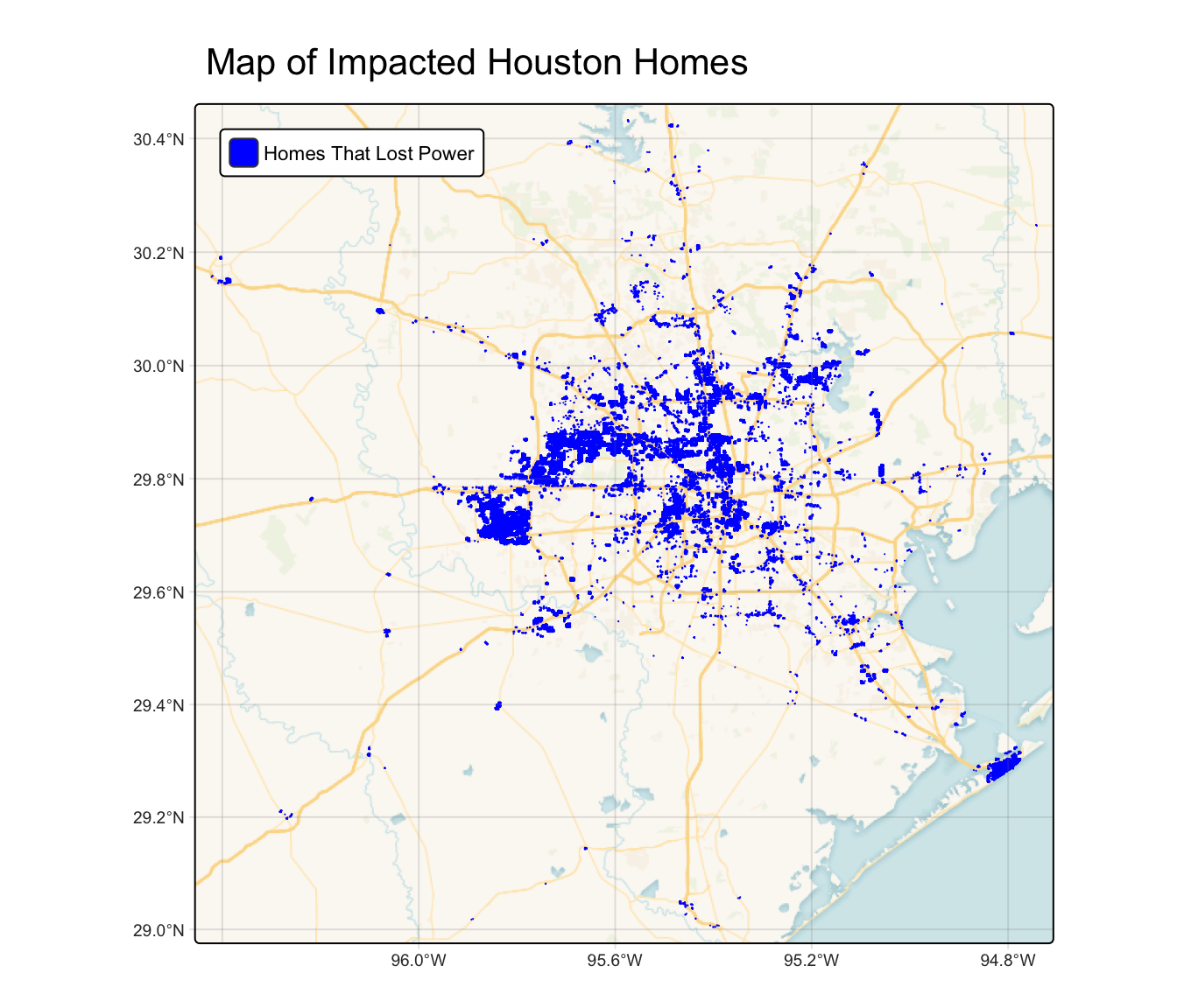
Code
# Table of homes that experienced blackouts
homes_df <- homes_blackout |>
  group_by(type) |>
  summarise(count = n(),
            percent = round((n() / nrow(homes_blackout)) * 100, digits = 2)) |>
  st_drop_geometry()

# Add total row
homes_df <- homes_df |>
  add_row(type = 'Total', count = sum(homes_df$count))

# Change type NA to character string
homes_df$type[6] <- "NA"
Code
# Display kable table
options(knitr.kable.NA = "")
kbl(homes_df,
    col.names = c("Home Type", "Count", "Percentage (%)"),
align = 'c')| Home Type | Count | Percentage (%) |
|---|---|---|
| apartments | 1136 | 0.72 |
| detached | 353 | 0.22 |
| house | 19760 | 12.51 |
| residential | 1395 | 0.88 |
| static_caravan | 80 | 0.05 |
| NA | 135246 | 85.61 |
| Total | 157970 |
Identify Census Tracts Impacted by Blackouts
In the same way as finding homes impacted, we use census data and our blackout areas to estimate the number of census tracts impacted and map them.
Code
# View layers in gdb file
#st_layers(here::here('data', 'ACS_2019_5YR_TRACT_48_TEXAS.gdb'))

# Extract income layer
income <- st_read(here::here('data', 'ACS_2019_5YR_TRACT_48_TEXAS.gdb'),
                  layer = 'X19_INCOME', quiet = TRUE) |>
  dplyr::select(c(GEOID, B19013e1, B19013m1))

# Extract census tract layer
census <- st_read(here::here('data', 'ACS_2019_5YR_TRACT_48_TEXAS.gdb'),
                  layer = 'ACS_2019_5YR_TRACT_48_TEXAS', quiet = TRUE) |>
  dplyr::select(-c(GEOID)) |> # Drop GEOID column
  rename(GEOID = GEOID_Data) |>  # Rename GEOID_Data for joining
  st_transform("EPSG:3083")
Code
# CRS check before joining & cropping
if (st_crs(houston_bbox) == st_crs(census)){
  print("CRS Match. Ready to find difference.")
} else {
  warning("Converting houston_bbox CRS to census CRS:\n", st_crs(census))

  houston_bbox <- st_transform(houston_bbox, crs = st_crs(census))
}

# Join census & income data
census_income <- left_join(x = census, y = income, by = "GEOID") |>
  st_crop(houston_bbox) |>
  filter(ALAND != 0) |>  # Filter out ocean geometries
  dplyr::select(c("GEOID", "B19013e1", "B19013m1")) |>
  rename(median_hh_income_est = B19013e1,
         median_hh_income_moe = B19013m1)
Code
# Filter to census tracts that lost power
census_blackouts <- census_income |>
  st_filter(y = blackout_far_areas, .predicate = st_intersects) |>
  mutate(blackout = TRUE) # Add blackout column

# Create blackout GEOID for filtering census_income & joining later
blackout_ids <- census_blackouts$GEOID
Code
# Create boolean column whether tract had a blackout or not
census_blackout_tf <- census_income |>
  mutate(blackout = GEOID %in% blackout_ids)
# Get value counts for blackout column & display table
blackout_table <- census_blackout_tf |>
  st_drop_geometry() |>
  group_by(blackout) |>
  summarise(count = n()) |>
  pivot_wider(names_from = blackout,
              values_from = count) |>
  mutate(total = rowSums(across(everything())))
Code
blackout_table |>
  kbl(col.names = c("No Blackout", "Blackout", "Total Census Tracts"),
align = 'c')| No Blackout | Blackout | Total Census Tracts |
|---|---|---|
| 191 | 935 | 1126 |
Code
# Plot blackout areas with census blackouts
tm_shape(census_income) + # Census layer
  tm_polygons() +
tm_shape(census_blackouts) + # Census blackout layer
  tm_polygons(fill = 'orange') +

tm_compass(position = c(0.92, 0.32)) +
tm_scalebar(position = c(0.76, 0.18)) +
tm_add_legend(labels = c("Tracts That Lost Power"),
              fill = c('orange'),
              type = 'polygons',
              position = c('right', 'bottom')) +
tm_title("Map of Impacted Houston Census Tracts")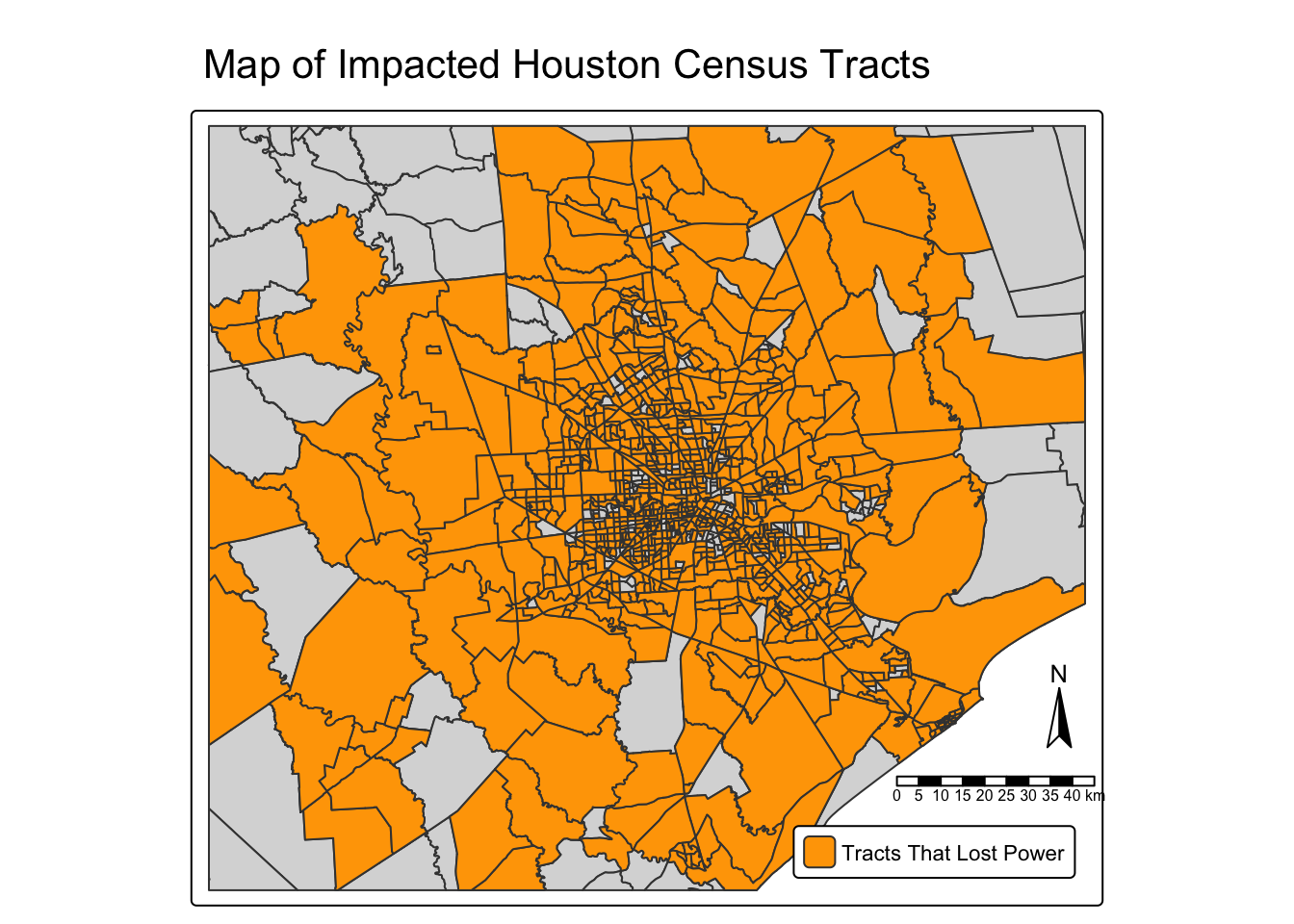
Combining median household income of each census tract and our impacted/non-impacted census tracts, we can display the distribution of income for each group.
Code
# Median household income plot
ggplot(census_blackout_tf, aes(blackout, median_hh_income_est)) +
  geom_boxplot() +

  scale_x_discrete(labels = c('No Blackout', 'Blackout')) +
  labs(title = "Distribution of Median Household Income for Census Tract Blackout Groups",
       y = "Median Household Income (Estimate) in Census Tract") +

  theme_classic() +
  theme(panel.grid.major.y = element_line(color = 'grey'),
axis.title.x = element_blank()) 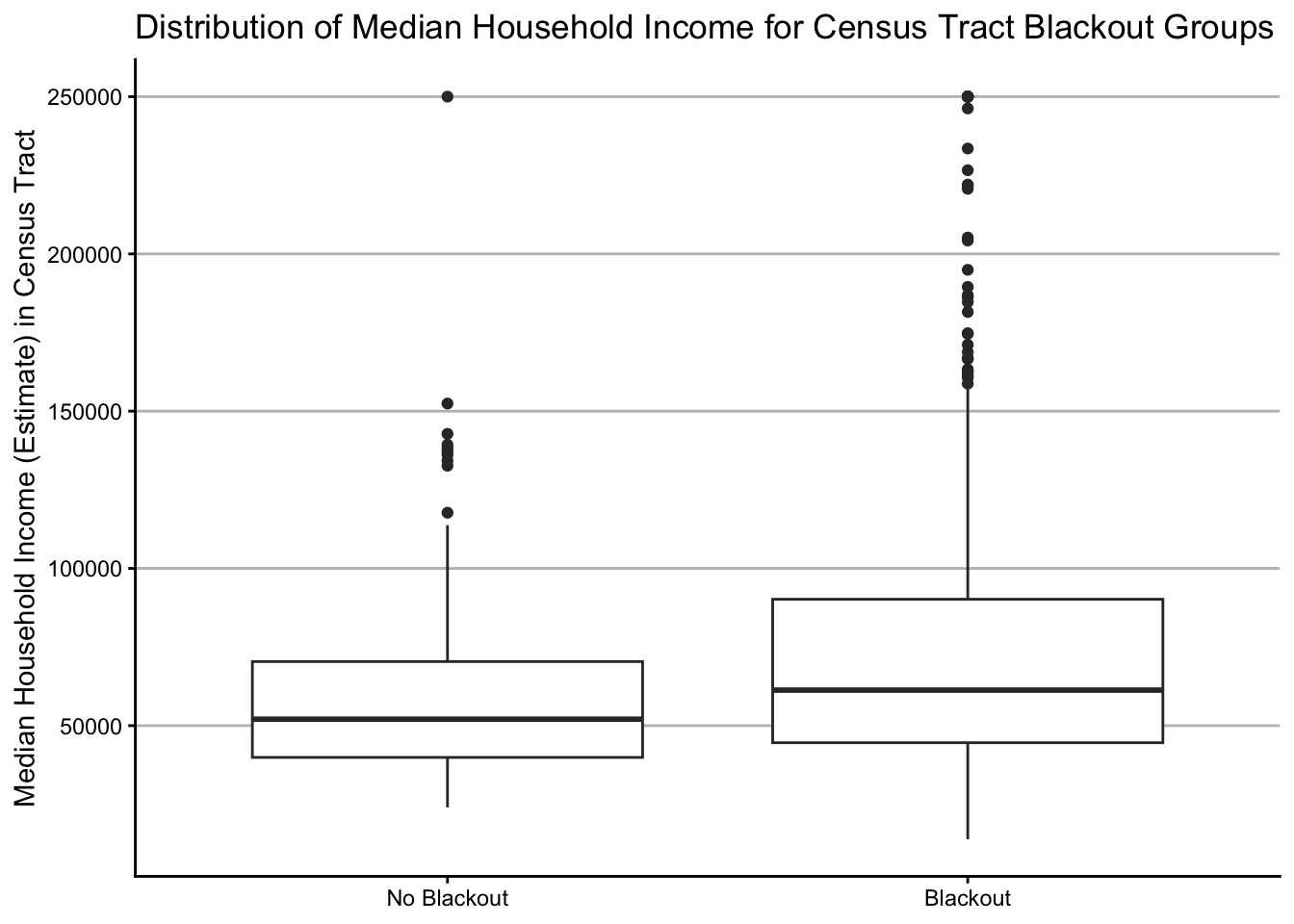
Summary
Winter storm Uri hit Texas in February 2021 and impacted over 100,000 homes within about 900 census tracts. It is documented that impacted census tracts did in fact have lower median household incomes on average, indicating that low-income communities in Texas were disproportionately affected by the storm (Lee et al. 2022). However, the boxplots in Figure 4 don’t show the expected results. One possible cause for this was the limited amount of data of only 2 days that was used in creating the blackout mask. Perhaps if we had more night light data spanning a range of dates, we could have a more accurate picture of what areas experienced blackouts, thus leading to a more historically accurate conclusion. Additionally, Lee et al. 2022 also faced data limitations as detailed power outage data was not available. Instead, the authors used data from Mapbox Population Activity, the 311 Houston Service Helpline, and SafeGraph POI Visit Data, along with the ACS census tract data to assess community impacts. While night light data provides a broad view of power outages across large areas, the alternative datsets in Lee et al. 2022 proved more effective in revealing the fine details and impacts of the storm.
References
Lee CC, Maron M, Mostafavi A. (2022). Community-scale big data reveals disparate impacts of the Texas winter storm of 2021 and its managed power outage. Humanit Soc Sci Commun. 2022;9(1):335. doi:10.1057/s41599-022-01353-8. Epub 2022 Sep 24. PMID: 36187845; PMCID: PMC9510185.
NASA. Extreme Makeover: Human Activities Are Making Some Extreme Events More Frequent or Intense - NASA Science. 8 Nov. 2021, https://science.nasa.gov/earth/climate-change/extreme-makeover-human-activities-are-making-some-extreme-events-more-frequent-or-intense/.
OpenStreetMap Contributors (2025). OpenStreetMap database. Retrieved from https://www.openstreetmap.org. Distributed by Geofabrik GmbH, Karlsruhe, Germany. Available at https://download.geofabrik.de/
Román, M.O., Wang, Z., Sun, Q., Kalb, V.L., Miller, S.D., Molthan, A., Schultz, L., Bell, J., Stokes, E.C., Pandey, B., et al. (2018). NASA’s Black Marble nighttime lights product suite (VNP46). Remote Sensing of Environment, 210, 113-143. https://doi.org/10.1016/j.rse.2018.03.017
U.S. Census Bureau. (2020). TIGER/Line Shapefiles and American Community Survey 2019 (5-Year Estimates), Texas — Census Tract Level (ACS_2019_5YR_TRACT_48_TEXAS) [Data set]. U.S. Department of Commerce. Available from https://www.census.gov/geographies/mapping-files/time-series/geo/tiger-data.html